Simple comparison of training time and performance of Extreme Learning Machines and regular feed forward network using Julia language.
With the advent of powerful computation techniques, there has been increasing interest back in the good old neural networks as major potential machine learning candidate after a long hiatus.
Modern and complex neural networks have come to the front, led by those dubbed Deep Learning Networks. Deep Learning algos are hot these days, thanks to the media. Just head over to datatau and you will know what I mean (btw I am not saying that they aren't worth the hype).
DL networks are basically networks with very deep (many) hidden layers in neural nets. One major problem with them is (as expected) of speed. Deeper hidden layers lead to deadly slow training time and the risk of overfitting. But recent works by Hinton and others in unsupervised feature learning have given a hefty lift to deep learning.
1. Reservoirs
But, this post is not about Deep Learning. Its about a different concept. A network that avoids the murky computation.
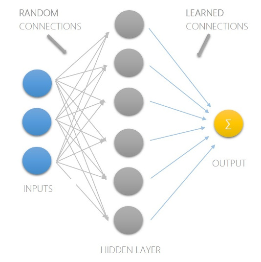
Recently, I came across the concept of Reservoir computing, which (in a very simple way) refers to a construct where the input are connected randomly to higher level of abstraction (see it as a hidden layer of higher level) and output can be tapped from those nodes and the training problem reduces to calculating the connection (weights) of tapping nodes to output. This avoids the major bottleneck, iterative tuning of weights of input to higher level.
Well, does this thing even work? Yes, farely well!
There is a concept known as Liquid State Machine, and a relatively better known Echo State Network which is used for training Recurrent Neural Nets. Both of them are based on reservoir computing. On the lines of reservoir computing and very similar in concept is the topic of this post, Extreme Learning Machine.
2. Extreme Learning
Extreme learning machine (ELM) is a modification of single layer feedforward network (SLFN) where learning is quite similar to the reservoir topic discussed above.
Given below is a simple SLFN with 3 inputs and 1 output which computes the weighted sum of hidden nodes.
After performing the tedious backpropagation ritual, we are left with the following equation that predicts output from inputs
\[ y = \sum h_i \]
Where \(h_i\) is the activation of \(i^{th}\) hidden neuron computed using
\[ h_i = f(\sum_j (w_{i, j} \times x_j) + b_i) \]
Here, \(f\) is the activation function like sigmoid, tanh etc., \(x\_j\) is the \(j^{th}\) input, \(w\_{i, j}\) is the connection weight from \(j^{th}\) input to \(i^{th}\) hidden neuron and \(b\_i\) is the bias term.
In matrix notation, the process can be represented in the following form
\[ Y = W' \times H \]
Where \(W'\) is the matrix of weights from hidden to output layer while \(H\) is the activation matrix computed using
\[ H = f(W \times X + B) \]
with \(W\) is matrix of weights from input to hidden layer.
Now, being different from usual SLFN, the ELM doesn't tune \(W\) using backprop or any other iterative method, instead \(W\) is randomly generated. This gives us a pool of higher level input abstractions in the hidden layer, out of which, ones fitting to training data can be found by adjusting hidden to output weights by solving a simple matrix equation.
\[ Y = W' \times H \]
Now, given a training data with \(X\) as input and \(Y\) as output, the ELM training process takes the following steps
- Generate \(W\)
- Find \(H\)
- Solve \(Y = W' \times H\) for \(W'\)
The value of \(W'\) can be calculated simply using psuedo (Moore-Penrose)
inverse which is usually available as a function that goes by the name pinv
most of the scientific computation environment including Matlab and Python's
numpy.linalg.
\[ W' = Y \times pinv(H) \]
This inverse can also be computed using regularized inverse for better generalization.
3. Performance
Let's test out the thing.
I happen to believe that we don't need slow languages
Enough to make me try julia.
For python users (for anyone, almost), like me, switching is ridiculously easy and fun. Although still in cradle, julia features nice set of basic libraries for scientific computing. Kinds of DataFrames, Gadfly and IJulia will make you feel at home, whether you are coming from R, scientific Python or Matlab / Octave.
And what you get? Speed, raw and visible! Calling C or fortran from python or R doesn't feel great, especially if you can avoid that.
Coming back to testing. While trying out julia, I coded a simple ELM library. I will be using that, and for comparison with regular NNs, I will be using the ANN library by Eric Chiang. In fact, this post is very much on the lines of a great post by Eric on yhat here.
The problem I will be taking is of a two class classification using the banknote authentication dataset. You can download the dataset and see its attributes here.
Starting off by installing required libraries
Pkg.clone("git://github.com/lepisma/ELM.jl.git");
Pkg.clone("git://github.com/EricChiang/ANN.jl.git");

import ELM, ANN;
Since, both libraries have few functions with same names, so its better to use
import rather than using.
3.1. Reading data
Pkg.add("DataFrames");
using DataFrames;

# No column names here :(
dat = readtable("data_banknote_authentication.txt", header = false);
head(dat)
6x5 DataFrame:
             x1      x2      x3       x4 x5
[1,]     3.6216  8.6661 -2.8073 -0.44699  0
[2,]     4.5459  8.1674 -2.4586  -1.4621  0
[3,]      3.866 -2.6383  1.9242  0.10645  0
[4,]     3.4566  9.5228 -4.0112  -3.5944  0
[5,]    0.32924 -4.4552  4.5718  -0.9888  0
[6,]     4.3684  9.6718 -3.9606  -3.1625  0
Last column is either 0 or 1 and tells us about the result of banknote authentication.
3.2. Scaling columns
Scaling all attributes to a similar scale makes sure that one attribute doesn't overshadow others.
# For all four columns
for i in 1:4
    # Subtracting the mean and dividing by standard deviation
    dat[i] = (dat[i] - mean(dat[i])) / std(dat[i]);
end
Keeping 20% of data for testing
n_test = int(length(dat[end]) * 0.2);
train_rows = shuffle([1:length(dat[end])] .> n_test);

dat_train, dat_test = dat[train_rows, :], dat[!train_rows, :];
3.3. Training
Let's create the models for training.
ann = ANN.ArtificialNeuralNetwork(10);
#10 hidden neurons, single hidden layer

elm = ELM.ExtremeLearningMachine(10);
#10 hidden neurons
Although ELM is also given 10 neurons, but since ELMs select from a pool, its better to give more options. But, whatever, the ultimate aim is to find the difference in training time of both when they provide almost similar accuracy.
Like Matlab, you can time your code in julia using tic() and toc()
functions. Before that, let us make functions for calculating accuracy.(Both
libraries return values in different ways)
# For ANN
function accu(model::ANN.ArtificialNeuralNetwork,
                      x_test::Matrix{Float64},
                      y_test::Vector{Int64})

    outputs = ANN.predict(model, x_test);
    predictions = Array(Int64, length(y_test));

    for i in 1:length(y_test)
        predictions[i] = model.classes[indmax(outputs[i, :])];
    end

    mean(predictions .== y_test)
end

# For ELM
function accu(model::ELM.ExtremeLearningMachine,
                         data_test::DataFrame)

    #ELM.jl supports DataFrames now !

    predictions = ELM.predict(model, data_test[1:end-1]);
    mean(int(predictions) .== data_test[end])
end
Back to training. After a bit of experimentation, following approach (basically, the choice of epochs in ANN) provides similar accuracy and a result that clearly shows the difference.
A word of caution : Since julia uses JIT compilation, it needs a bit of warm up. So, the first call to functions doesn't show the actual speed of julia.
3.4. ANN
tic(); ANN.fit!(ann, array(dat_train[1:end-1]), array(dat_train[end]), epochs =
                16, lambda = 1e-5); toc()
accu(ann, array(dat_test[1:end-1]), array(dat_test[end]))
elapsed time: 0.238218045 seconds
0.9708029197080292
3.5. ELM
tic(); ELM.fit!(elm, dat_train[1:end-1], dat_train[end]); toc()
accu(elm, dat_test)
elapsed time: 0.003801902 seconds
0.9817518248175182
4. WUT?
Assuming both models give same accuracy, the training of ELM is around 60x faster than ANN! (Which kind of isn't actually surprising since the hidden connections are untouched).
- As pointed out by Jeremy Gore, the current code throws error due to changes in Julia version. The original post was tested and written for Julia v0.2. I will update the post to meet the updated Julia standards after I get free from a few things I am currently in.
- The library (and this post) is updated to work with newer Julia versions (tested on v0.3.3) with added support for DataFrames.
- I thought to include my personal thoughts (which have also changed
since I first wrote the post) on ELMs since there are unbelievably
large amount of misconceptions popping everywhere on the internet.
- As it is obvious, there is just one hidden layer and the whole ideas centers around creating random projections of input to finally solve a linear equation problem. This can not be justified as a solution for hard and complex problems of the class currently tackled beautifully by deep learning methods.
- Talking about the originality of the concept of random projections, I personally am not a science historian (at least not right now) and would prefer the reader to do his/her own research.
- The main thing that looked promising to me here was the idea that tapping from random projections can solve a class of problems. This might not be charming enough for anyone else, or even me at a different spot in space-time, but anyways, I did a simple comparison and posted the stuff here.